A practical adiabatic (0PA) flux workflow for generic EMRIs
This note introduces a practical workflow for large scale 0PA flux generation: a reusable radial solver layer, a tail aware mode summation order, and Adaptive Levin integration for difficult source integrals in generic EMRI calculations.
In EMRI waveform work, a flux calculation is rarely a one time exercise. One quickly ends up with many parameter points, many modes, and orbits that may be eccentric, inclined, or close to difficult regions of Kerr parameter space. The useful question is therefore not only “can I compute this mode?” It is: can I compute many modes, see where the truncation really happens, reuse the expensive pieces, and avoid wasting samples on oscillations that the integrator should understand analytically?
The main bottlenecks show up in three connected places. First, every mode needs a radial Teukolsky solve, so the radial solver quickly becomes the most expensive repeated operation. Second, the mode sum itself is hard to truncate if the calculation simply grows a rectangular block in $(\ell,m,k,n)$ space. Such a block may include many modes with negligible flux, while missing modes outside the block that still matter, which can underestimate the total flux. Third, the slow radial tail means that large $n$ modes must be evaluated, and those modes lead to highly oscillatory convolution integrals.
The workflow follows these bottlenecks one by one. The radial equation is handled by an iterative series expansion matching method, ISEM for short. The mode sum is reorganized so that the important angular structure enters first and the radial harmonic $n$ remains visible as the final tail direction. When the tail produces strongly oscillatory source integrals, the calculation switches to Adaptive Levin integration.
Motivation: why this is worth doing
LISA, Taiji, and TianQin are space based gravitational wave detector projects. One important class of sources for these missions is EMRIs, where 0PA flux generation becomes a production scale numerical task rather than a small script. Frequency domain Teukolsky calculations are accurate and modular, but the cost grows sharply when the orbit becomes highly eccentric, inclined, and precessing. In the fully generic case, the signal power is spread across a large set of $(\ell,m,k,n)$ modes. If the time for a single mode cannot be reduced effectively, the full flux calculation becomes a large computational expense.
The goal is not only to compute one mode quickly. The goal is to know which part of the spectrum is still active, which part has become tail, and which numerical method should be used for each region. That is where the current implementation differs from a plain rectangular mode loop: it treats the mode sum as something to diagnose, not just something to force through a larger grid.
The radial solver layer
The first piece is the radial solver. Here the radial Teukolsky equation is handled by iterative series expansion matching, abbreviated as ISEM below. The idea is to use the transformed form of the Teukolsky equation, build series expansions from the horizon and from infinity, and then propagate the two physical branches toward an intermediate matching point. At that point, the solution and its radial derivative are matched to determine the matching coefficients, which are also the asymptotic amplitudes needed for flux evaluation. The full radial solution is then reconstructed from the matched branches.
This is the right place to spend effort because the radial solve sits inside every mode calculation and has long been a bottleneck in the source integral calculation. In the current implementation, this construction is roughly two orders of magnitude faster than the traditional direct numerical GSN solve and MST based routes for the same repeated mode production use case. Reducing this cost for each mode is what makes the larger 0PA flux workflow practical.
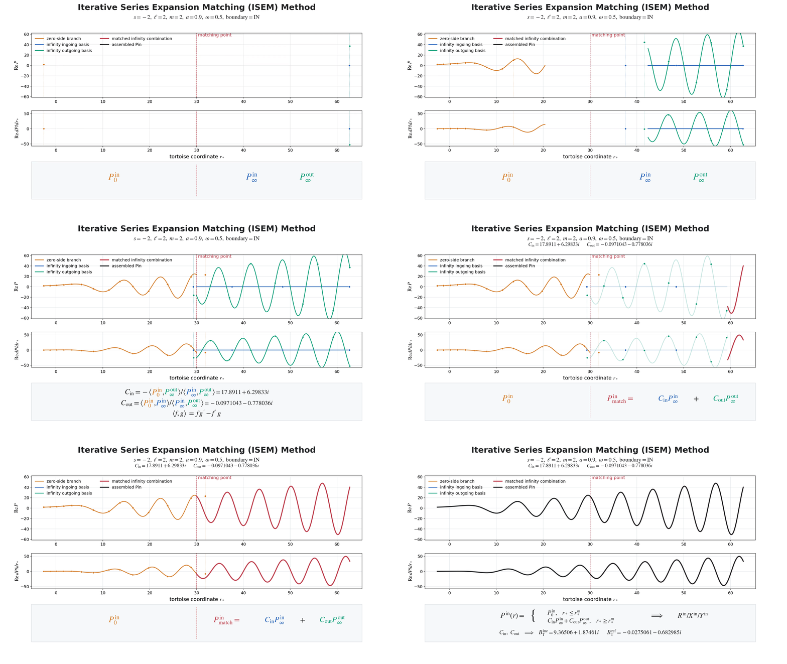
Build horizon side and infinity side homogeneous radial Teukolsky solutions from controlled series expansions.
Match the solution and derivative at an intermediate point to obtain the asymptotic amplitudes.
Reuse the reconstructed radial solution and amplitudes in the source integral and flux evaluation.
How modes are added together
Next comes the mode summation order. The useful empirical structure is that the largest contributions usually sit close to the diagonal in angular space: for a fixed $\ell$, modes with $m=\pm \ell$ are often among the dominant branches. A direct rectangular loop does not exploit this structure. If one fixes $\ell$ and then scans all $m$ from $-\ell$ to $\ell$, and then repeats this inside large $k$ and $n$ ranges, the calculation can spend many modes before the relevant convergence pattern becomes clear.
A more useful order is to fix $m$ and grow $\ell$ from $\max(\mathrm{abs}(m),2)$ upward. This makes the angular convergence easier to see. The same idea can then be extended to the polar and radial harmonics. The $k$ direction often converges quickly, usually within about ten shells for the cases considered here, while the radial harmonic $n$ is slower and carries the long eccentricity tail. For that reason, $n$ is left as the final summation direction.
The older mental model is:
Rectangular grid mindset
- Choose a large box in (ℓ, m, k, n).
- Loop through the full block even when many entries are already negligible.
- The slow radial tail is mixed into the whole four dimensional rectangle.
Production workflow mindset
- For each m, grow ℓ from max(abs(m), 2) upward.
- Add the faster k shells before the slow radial direction.
- Leave n last, so the eccentric tail truncation is visible.
The practical advantage is that convergence becomes easier to diagnose. Instead of asking whether a whole rectangular block is large enough, the code can report where the infinity and horizon branches reached in $n$, how large the final shell contribution is, and whether $n_\mathrm{max}$ should be increased. In this ordering, the maximum radial truncation used in the code is $n_\mathrm{max}=500$, which is stable for the target cases with $e<0.9$. Compared with the rectangular ordering, this shell aware order typically reduces the number of modes that need to be evaluated by about 50%, while making the truncation decision more transparent.
The resulting workflow is therefore $\ell \to m \to k \to n$: angular structure first, the fast polar direction next, and the slow radial tail last. This is not just a different loop order; it is a way to expose the convergence information that is otherwise hidden inside a large rectangular sum.
Adaptive Levin: use the right tool for the tail
The third piece is Adaptive Levin integration. In generic 0PA flux calculations, source integrals with large $n$ can oscillate rapidly. A plain quadrature rule then pays for many samples whose job is just to chase phase. In representative one dimensional radial integrations, a standard sampling route may need about $2^{14}=16384$ radial samples to reach the desired convergence, while the Adaptive Levin route can reach the same convergence with an effective scale closer to $2048$.
The Levin method treats a highly oscillatory integral by rewriting it as an auxiliary ODE system; after discretization, that system becomes a small matrix solve. The adaptive part is a bisection refinement of the integration interval: easy regions stay coarse, while difficult oscillatory regions are split into smaller segments. On each local segment, Levin itself only needs a small one dimensional collocation grid, typically $q=17$, rather than a very fine sampling mesh. The dense local solve scales roughly like $O(q^3)$ per segment, and the total cost follows the number of accepted segments. For generic two dimensional integrals, the current route uses Adaptive Levin in the radial direction and Clenshaw Curtis quadrature in the $\theta$ direction.
The effect is simple: the difficult high $n$ integrals no longer require the same brute force sampling strategy as the easy modes. Radial Adaptive Levin plus fixed $\theta$ direction Clenshaw Curtis keeps the high frequency radial direction under control, while still using a stable tensor product structure for generic orbits.
Related software and modules
- GeneralizedSasakiNakamura.jl: current ISEM development branch.
- KerrGeodesics.jl: bound Kerr geodesic infrastructure for orbital frequencies, phases, and trajectories.
- AdaptiveLevin.jl: adaptive methods for highly oscillatory integrals.
- Tools overview: homepage entry point for the software modules.